Reverse Engineering the Hacker News Ranking Algorithm
All data and code used in this article can be found on GitHub.
Introduction
Articles occasionally pop up on Hacker News that analyze historical data relating to posts and comments on the site. Some of the analyses have been quite interesting but they almost universally focus on either basic metrics, content analysis, or how to get on the front page. Every time I read one of those articles, it always gets me wondering about what the same data could tell us about how Hacker News actually works.
There are a lot of questions one could ask but one of the most obvious is: what determines the position of stories on the front page? I find this to be a particularly interesting question, not because I actually care about the answer, but because it feels like the data should be able to tell us the answer. We could of course pick some different models and use the historical data to fit and validate them… but this isn’t what I mean. I just have this feeling that the data can actually tell us the answer in a more direct way than global optimization.
What follows is an exploration of how we can use the data to learn about how the algorithm works. It shouldn’t be confused with an attempt to find the best predictor for the front page rank, there are better ways to do that. My main goal was to tease out the ranking algorithm from the data in a simple and elegant fashion. This made it a little more interesting as an endeavor and hopefully makes it a more interesting read as well.
When You Make Assumptions
Anybody who reads Hacker News with any regularity probably has some rough but intuitive understanding of how the ranking algorithm works. If you’ve ever seen a story and thought “jeez, this must have been flagged a lot to be this far down the page” then you were basically predicting where it should appear and then noticing a discrepancy from that. Here are a few examples of my guess-timations of where a story might appear on the front page.
| votes | age | position # |
|---|---|---|
| 15 | 41 minutes | 8 |
| 140 | 21 minutes | 2 |
| 3000 | 4 days | > 30 |
| 500 | 12 hours | 15 |
| 40 | 8 hours | 28 |
I doubt that anybody is going to start calling my psychic hotline after seeing me make these guesses but it’s actually pretty interesting that we can make even rough predictions. I think that this implies that we have some underlying beliefs about how the ranking algorithm works. Some of these might be things that we just feel must be true while others are more heavily supported by observations. When I approach a new problem, I like to start by clarifying any implicit assumptions and then seeing if I can use them to build a more structured approach.
One very general assumption that I made when coming up with those predictions was that the rank is primarily determined by a story’s vote total and its age which we’ll denote with $v$ and $t$ respectively. I know that there are contributions from flagging, @dang boosting stories, spam detection, etc. but I expect these to be somewhat secondary in most cases and we don’t have access to their corresponding variables anyway. Another broad assumption is that $v$ and $t$ are used to calculate some numerical score and that the stories are ranked by sorting their scores. We’ll represent this score function as $\mathcal{F}(t, v)$.
Having a general framework for how the ranking works, we can move to thinking about $\mathcal{F}(t, v)$ itself. Let’s start with how the score changes with age. Here’s how I classify some guesses regarding the age dependence of the score.
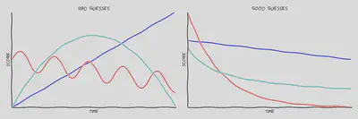
There are two main things I consider when judging these different curves. First off, it doesn’t really make sense for the score to get higher as a story gets older; you don’t see stories from a few months ago hopping back onto the front page for no reason. I’m assuming that the score must decrease as $t$ decreases and for a fixed $v$. Mathematically, this is equivalent to saying that the partial derivative $\frac{\partial \mathcal F}{\partial t} < 0$.
The second assumption is more subtle: small differences in age make less of a difference for large $t$. The difference between ages of one hour and eleven hours will have a huge impact on the score while the difference between one year and one year plus ten hours should be pretty negligible. This means that the score curves upwards as a function of $t$ and therefore $\frac{\partial^2 \mathcal F}{\partial t^2} > 0$.
We can apply similar reasoning to the dependence of $\mathcal F(t, v)$ on the number of votes $v$. I expect more votes to always mean a higher score so we can conclude that $\frac{\partial \mathcal F(t, v)}{\partial v} > 0$. My first guess would be that $\mathcal F(t, v)$ is proportional to $v$ but I could imagine somebody wanting to slightly suppress the growth for very large $v$ because stories that are on the front page for longer will get seen by more people and will therefore get even more votes. There’s a multiplicative effect here and you could counteract this by introducing downwards curvature with something like $\mathcal F(t, v) \propto v^{\frac 1 2}$. Any functions that suppress this effect will have $\frac{\partial^2 \mathcal F}{\partial v^2} < 0$ while functions with $\frac{\partial^2 \mathcal F}{\partial v^2} > 0$ would actually exacerbate it. We’ll assume that $\frac{\partial^2 \mathcal F}{\partial v^2} \le 0$ to allow for suppression but not enhancement of the effect.
I should probably mention now that these second derivative limits are a little bit over-simplified. It’s easy to see that multiplying the score function by a positive constant won’t affect the relative rank of stories but there are actually a much broader set of transformations that also won’t affect it. Given a score function $\mathcal F(t, v)$, you can apply any monotonically increasing transformation and get out another score function that has the same lexicographical sorting order. So if $\mathcal F(t, v) \propto v$ then $\mathcal F(t, v)^2$ will have upward curvature as a function of $v$ and violate our assumption that it shouldn’t. You can similarly apply transformations that would cause the $\frac{\partial^2 \mathcal F}{\partial t^2} > 0$ assumption to be violated.
What’s really going on here is that those limits need to be constructed with appropriate scaling factors in order to be invariant under all allowable transformations. I’m tempted to explain this more but it would add a lot of complexity to the discussion without really changing anything in the end. I think that the best balance to strike here is to just be aware that there’s a little more to the story but that there should exist a score function that still satisfies our constraints.
Working in Observations
So to summarize the last section, these are what we’re going to accept as absolute truth:
- $\mathcal{F}(t, v) $ - The score function used to rank stories.
- $\frac{\partial \mathcal F}{\partial t} < 0$ - It decreases over time.
- $\frac{\partial^2 \mathcal F}{\partial t^2} > 0$ - It curves upwards over time.
- $\frac{\partial \mathcal F}{\partial v} > 0$ - It increases with votes.
- $\frac{\partial^2 \mathcal F}{\partial v^2} \le 0$ - It curves downwards with votes.
Now let’s see what they can buy us.
Anything further is going to need to be tied to actual observations on how stories are ranked. Fortunately, this is something that we can easily observe by visiting the website. Say that we observe two stories on the front page and Story 1 appears in a better position than Story 2. This tells us that Story 1 has a higher score than Story 2 or, more formally, $\mathcal{F}(t_1, v_1) > \mathcal{F}(t_2, v_2)$.
We now need to work in our assumptions somehow in order to make this statement more useful. If you’re a little rusty on your calculus then this chart might help to understand what we’re about to do.
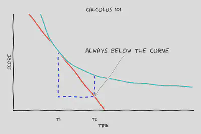
What’s plotted here is $\mathcal F(t, v)$ for some value of $v$, essentially reducing it to a one-dimensional function. The red line shows the tangent curve which just barely kisses $\mathcal F(t, v)$ at $t=t_1$ and has a slope of $\frac{\partial \mathcal F}{\partial t} \biggr\rvert_{t=t_{1}}$. The arrow points to $(t_2, \mathcal F(t_1, v) + (t_2 - t_1) \frac{\partial \mathcal F}{\partial t} \biggr\rvert_{t=t_{1}})$ and it’s noted that this point is always below $(t_2, \mathcal F(t_2, v))$. This would not always be true if the score could curve downwards with time but this is forbidden by Assumption 2 and so we can safely conclude that $\mathcal F(t_1, v) + (t_2 - t_1) \frac{\partial \mathcal F}{\partial t} \biggr\rvert_{t=t_1} < \mathcal F(t_2, v)$. Plugging this back into our relationship between the scores of the two observed stories results in
$$\mathcal F(t_1, v_1) > \mathcal F(t_1, v_2) + (t_2 - t_1) \frac{\partial \mathcal F}{\partial t} \biggr\rvert_{t=t_1,v=v_2}$$
A similar inequality for the extrapolation as a function of $v$ follows from Assumption 5: $\mathcal F(t, v_2) + (v_1 - v_2) \frac{\partial \mathcal F}{\partial v} \biggr\rvert_{v=v_2} \ge \mathcal F(t, v_1)$. The direction of the inequality is opposite here because $g(v)$ curves downwards instead of upwards but otherwise it’s the exact same concept. We can now plug this into the left hand side to get
$$\mathcal F(t_1, v_2) + (v_1 - v_2) \frac{\partial \mathcal F}{\partial v} \biggr\rvert_{t=t_1,v=v_2} > \mathcal F(t_1, v_2) + (t_2 - t_1) \frac{\partial \mathcal F}{\partial t} \biggr\rvert_{t=t_1,v=v_2}$$
which simplifies to
$$(v_1 - v_2) \frac{\partial \mathcal F}{\partial v} \biggr\rvert_{t=t_1,v=v_2} > (t_2 - t_1) \frac{\partial \mathcal F}{\partial t} \biggr\rvert_{t=t_1,v=v_2}$$
OK, that’s basically it! We now have an equation that translates our assumptions into a simple relationship that can be used to determine $\mathcal F(t, v)$. Each observation further constrains a differential equation that can then be solved to find $\mathcal F(t, v)$. This could be done directly but things will be much easier if we introduce an additional assumption here that the relative rate of score decay as a function of $t$ is independent of $v$. That makes the differential equation separable and so there exists a solution of the form $\mathcal F(t, v) = f(t)g(v)$. This will just make it easier to visualize and discuss, it’s otherwise not a necessary assumption.
Substituting in this separable form of the score function gives us
$$-\frac{f(t_1)}{f^\prime(t_1)} > \frac{(t_2 - t_1)}{(v_2 - v_1)} \frac{g(v_2)}{g^\prime(v_2)}$$
when $v_1 > v_2$ or with a $<$ sign instead of a $>$ sign when $v_2 > v_1$. Note that we also implicitly used Assumptions 2 and 4 here to swap the equality sign appropriately when dividing or multiplying by negative quantities.
The general approach that we’ll now take is to choose an ansatz, or reasonable guess, for $g(v)$ and then use that to determine an estimate for $f(t)$. We can then turn around and use this estimate of $f(t)$ to figure out a better guess for $g(v)$. If we repeat this process then things should hopefully settle down to satisfactory functions for $g(v)$ and $f(t)$. This lets us deal with differential equations of a single variable for simplicity.
Let’s use $g(v)=v$ as our initial ansatz. It’s simple, satisfies our assumptions, and is probably what I would have picked if I had programmed Hacker News. Given this ansatz we find that our inequality simplifies to
$$-\frac{f(t_1)}{f^\prime(t_1)} > v_2\frac{(t_2 - t_1)}{(v_2 - v_1)}$$
where the direction of the inequality again depends on whether or not $v_1 > v_2$. To avoid writing that left hand side over and over let’s define $\tau(t) \equiv \frac{f(t)}{f\prime(t)}$ which then reduces our bound equation to
$$\tau(t_1) > v_2\frac{(t_2 - t_1)}{(v_2 - v_1)}$$
Let’s take a minute to step back and see what this equation is really telling us. To simplify things a bit, we’ll briefly consider the case of exponential decay $f(t)=e^{-t/\tau_0}$ where larger values of $\tau_0$ mean that stories fall off the front page more slowly. This isn’t an assumption that we’ll use in the analysis; we’ll just use it to develop some intuition about what the bounds mean. We can then see that $\tau(t) = \frac{f(t)}{f\prime(t)} = \tau_0$ so our inequalities are going to be directly constraining $\tau_0$ regardless of $t$. The exact nature of the constraint is going to depend on whether $v_1>v_2$ and whether or not $t_1>t_2$.
If $v_1 > v_2$ then we’ll be putting a lower bound on $\tau_0$. If $t_1$ is less than $t_2$ then this bound will be negative which doesn’t tell us much because $\tau_0$ has to be positive for exponential decay. This makes a lot of sense because a newer story with more votes has to have a higher score given Assumptions 2 and 4. Seeing that just confirms our assumptions, it doesn’t tell us anything further about $f(t)$. It gets more interesting when the top story is older than the lower story. That puts a positive lower bound on $\tau_0$ which means that if old stories were to fall off more quickly than the bound allows then Story 1 would have already fallen below Story 2.
On the other hand, if $v_1 < v_2$ then we’ll be putting an upper bound on $\tau_0$. If $t_1$ is less than $t_2$ then this bound will be negative which would mean that $f^\prime(t) > 0$, violating Assumption 2. Indeed, if Assumptions 2 and 4 hold then we would expect to never see the higher scored story be both older and have less votes so this issue should never come up. $t_1>t_2$ is the more interesting case because it means that the top story is newer but has less votes. This means that Story 2 must have started falling off with a small enough value of $\tau_0$ in order to come in second even though it has more votes.
Hopefully those examples make the bounds that we’re calculating a little more intuitive. The lower bounds eliminate faster decays while the higher bounds eliminate slower ones. The decay doesn’t need to be a constant value though, it can of course depend on $t$. If it does, then we’ll need to compute this bounds for different values of $t$ to get a more complete picture.
The Good
Now it’s just a matter of actually crunching some data to see what we find. I put together a dataset of front page snapshots from 2007 to 2017 that includes the vote total, age, and relative position of each story to use for this analysis. The stories are limited to those that link to external URLs in case self-posts are treated differently. You can grab the dataset, as well as the analysis code, from this GitHub repository if you would like to play along at home.
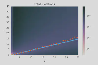
Let’s start out by just histogramming the upper and lower bounds that we observe. Each entry here is a bound on $\tau(t)$ obtained by evaluating the inequality that we derived earlier for two observed stories.
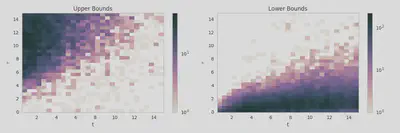
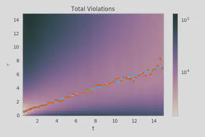
We can already see how these two histograms can work together to constrain $\tau(t)$. Let’s combine them and plot the number of bounds that a given value of $\tau(t)$ would violate as a function of $t$.
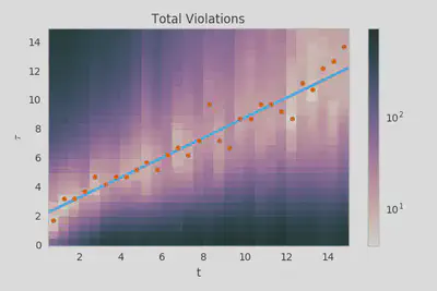
The points on this plot show the value of $\tau(t)$ for each $t$ bin that violates the fewest bounds. The line represents the $\tau(t) \approx \tau_0 + \tau_1 t$ fit that minimizes the total number of bounds that are violated. To my eye, this seems like a pretty reasonable fit and I don’t think that we could accurately constrain any higher order terms given the available data.
This differential equation described by this parameterization of $\tau(t)$ has a very simple solution
$$f(t)=(\tau_0 + \tau_1 t)^{-\frac{1}{\tau_1}}$$
Interestingly, you can see that the limit of this quantity as $\tau_1 \to 0$ is proportional to, and therefore equivalent to in terms of ranking, $e^{-t / \tau_0}$. This is the function we played around with when trying to develop some intuition about what the bounds mean and we found that $\tau(t)$ would be constrained to a constant value of $\tau_0$. We can think of the solution we found here as a generalization of exponential decay that adds another parameter to make the score fall off more slowly for larger values of $t$.
This plot of the bounds violations encompasses what I was talking about when I said that the data could tell us how the algorithm works. From just glancing at the figure, it’s obvious that the score decays as a power law with age and you can even pull out rough estimates for the parameters by eye: $\tau_0$ is about 2 hours and $\tau_1$ is about 0.75. There’s just something about that I find extremely satisfying.
Perhaps I’m getting ahead of myself a bit though… we said before that $g(v)=v$ was just a guess and that we would need to revisit it after we used it to constrain $f(t)$. Let’s flip it around now and use our newly determined function $f(t)$ to constrain $\frac{g(v)}{g^\prime(v)}$ which we’ll denote $\nu(v)$.
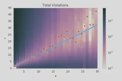
The line again represents a minimization of the total bound violations, this time parameterized as $\nu(v)=\nu_0 + \nu_1 v$. The fit parameters are $\nu_0=-0.41 \pm 0.31$ and $\nu_1=1.091 \pm 0.069$ where the errors are only statistical and were determined by bootstrapping the set of bounds on $\nu(v)$. These are both consistent with our ansatz of $\nu_0=0$ and $\nu_1=1$ which confirms that our ansatz was fairly accurate.
We could now try to iterate further using this solution but things are complicated by the fact that an arbitrary scaling factor can be applied to $\nu_1$ and $\tau_1$ without effecting the ranking properties of the score function. Unfortunately, the main thing that this would accomplish would be to let these parameters drift indiscriminately. If we had found non-zero curvature for $\nu(v)$ then we could have fixed the linear term to $1$ and then used the iterative process to determine the higher order terms. The only thing that we would be constraining in this linear case would be $\nu_0$ and it doesn’t seem like we have the resolving power to differentiate between $0$ and $-1$ so there isn’t much point in doing that.
Ultimately we conclude that the score function, or at least an equivalent score function is
$$\mathcal F(t, v) = \frac{v}{(\frac{\tau_0}{\tau_1} + t)^{\frac 1 \tau_1}}$$
with values of $\tau_0 = 1.95 \pm 0.16$ and $\tau_1 = 0.688 \pm 0.033$ extracted from the fit.
The Bad
I mentioned in the previous section that I put together a dataset of stories from 2007-2017. What I didn’t mention is that I was only showing you an analysis of data from 2007 and 2008. That’s partially because I wanted you to see this approach succeed before seeing it fail but it’s also because it’s a little easier to understand this next figure after walking through the analysis for a single time period.
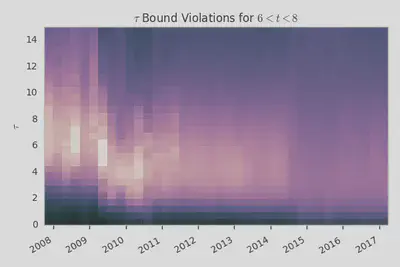
This figure shows the number of bound violations for different values of $\tau(t)$ within a window of $6 < t < 8$ for each three month period from mid 2007 until present. The columns are also normalized to give a consistent picture even though the amount of data varies over time.
It’s clear that $\tau(t)$ dropped significantly around the first quarter of 2009 which tells us that the score function was adjusted so that stories would drop off more quickly. It seems like maybe there were changes around mid-2010 and mid-2011 as well but it’s hard to tell exactly because the amount of data is also changing and this could just be shifts in the quantity of noise. What’s unmistakable, however, is that our valley of $\tau(t)$ values with relatively few bound violations gets demolished in mid-2014. This sort of change is what we would expect if our assumptions get seriously broken (e.g. by heavy-duty vote fuzzing).
I just want to take a second to emphasize that it’s really cool that the general approach we’ve taken allows us to visually see when these changes in the algorithm occur as well as their nature. That said, these algorithm changes unfortunately do mark a breakdown in some of our assumptions and that means that any results we pull out will become less accurate. Our approach is somewhat robust against factors like flagging and vote fuzzing: both of these will basically add noise to the upper and lower bound values which will cancel to leading order when determining the best values for $\tau(t)$ or $\nu(v)$. If additional factors become large enough that the lower and upper bounds overlap a lot though then the extracted fit parameters may be seriously biased. Just by eye, it’s clear that this will be the case for mid-2014 through present and there’s a good chance that it’s also the case for 2009 through mid-2014.
Let’s look briefly at what happens in the data after mid-2014. The $\tau(t)$ constraints actually aren’t that bad…
You could almost imagine how deconvolving that image would give back our nice clean valley but it’s not really possible to put too much faith in the extracted parameters. You can definitely rule out exponential behavior though and you can probably reasonably constrain $\tau_1$ to within a factor of 50% or so.
Where things get really bad is when we use the extracted $\tau(t)$ function to constrain $\nu(v)$.
The extracted value for $\nu_1$ is $0.52 \pm 0.01$ which isn’t consistent with our ansatz at all (and the first order terms agreement can’t be improved via iteration). What’s most likely happening here is that there are just way more upper bounds than lower bounds and the blurring effect introduced by vote fuzzing, story promotion, etc. are causing these to overwhelm the lower bounds and push the preferred $\nu(v)$ down significantly. If $g(v)$ is still equal to $v$ then maybe we can kinda sorta use our $\tau(t)$ constraints to determine $\mathcal F(t, v)$, but we really can’t do that with the same level of confidence that we did for the data from 2007-2008.
The situation for the 2009-2014 data has the same problem to a much, much lesser extent. This article already has more than enough figures so I won’t show the plots here but they’re included in the GitHub repository if you would like to see them. The extracted value for $\nu_1$ here is $0.81 \pm 0.02$ which is much better than in the 2014-2017 but still demonstrates some violation of our assumptions. Despite that, the valley is clearly defined and you can much more clearly see how it was shifted down. I would actually be willing to somewhat trust the $\tau(t)$ parameterization in this case while also recognizing that there are definitely additional factors at play.
An interesting thing to note here is that both of these later time periods suggest $v_0=-1$ rather than $0$. It’s a little hard to trust this coming from data where our assumptions clearly break down but with the 2007-2009 data being inconclusive and the 2009-2014 data looking not-actually-that-bad then it at least suggests the possibility of $g(v)=v-1$ where the nitial automatic self-vote doesn’t count.
(the ugly)
So you’ve seen the good and you’ve seen the bad. Now it’s time to see… code written in Arc. I kid ‘cause I love.
Anyway, there exists a sort of Bizarro Hacker News out there where everyone really loves lisp. OK, I guess that that applies to the real Hacker News too… but everybody there specifically loves Arc. For those of you who aren’t familiar: Arc is a dialect of Lisp developed by Paul Graham. The Arc Language Forum is a place for people to post and discuss stuff relating to Arc and it uses- or at least used at some point- basically the same code as Hacker News. More importantly, this code was included as part of the Arc distribution.
The first major Arc release was that of Arc 2 in February 2008 and it included the source for Hacker News in news.arc. The file is dated September 2006 though and presumably the file had been in use for the previous year before being released. The portion of the code relevant to the ranking algorithm is
; Ranking

; Votes divided by the age in hours to the gravityth power.
; Would be interesting to scale gravity in a slider.

(= gravity* 1.4 timebase* 120 front-threshold* 1)

(def frontpage-rank (s (o gravity gravity*))
  (/ (- (realscore s) 1)
     (expt (/ (+ (item-age s) timebase*) 60) gravity)))

(def realscore (i) (- i!score i!sockvotes))

(def item-age (i) (minutes-since i!time))
which, if you aren’t familiar with lisp, might be more comprehensible rewritten in python as
def frontpage_rank(story, gravity=1.4, timebase=120):
    effective_score = story.score - story.sockvotes - 1
    return effective_score / ((timebase + story.age) / 60)**gravity)
This is also equivalent to a score function
$$\mathcal F(t, v) = \frac{v - 1}{(\frac{\tau_0}{\tau_1} + t)^{\frac 1 \tau_1}}$$
where $\tau_1 = \frac{1}{1.4} \approx 0.714$ and $\tau_0 = \frac{120}{60}\tau_1 = 1.43$. Note that the initial self-vote is subtracted off so the $\nu_0=-1$ values that we got from the later time periods were likely correct (the early data was inconclusive). The vote total also subtracts off “sockvotes” which are presumably votes connected to spam accounts or vote rings. Other than that, our initial assumptions hold quite well and it’s unsurprising that we had such success with the early data.
Now that we know what the actual score function was, we can compare it to what we extracted using our differential equation approach. To make things more interesting, let’s also include the parameters extracted using global optimization over the data for two different cost functions. One is the Euclidean distance such that if the front page ordering is observed as $[1, 2, 3, 4]$ but predicted as $[1, 4, 3, 2]$ then the cost is $\sqrt{(1-1)^2 + (2-4)^2 + (3-3)^2 + (4-2)^2}=2$. The second is the Levenshtein distance applied to the same vectors. I won’t go into the details here but the Levenshtein distance will basically punish a story the same amount for being a little or a lot out of order (e.g. $[4, 1, 2, 3]$ and $[1, 2, 4, 3]$ are equivalently bad predictions).
| Actual | Diff-EQ | Euclidean | Levenshtein | |
|---|---|---|---|---|
| $\tau_0$ | $1.43$ | $1.95 \pm 0.16$ | $3.15$ | $3.34$ |
| $\tau_1$ | $0.714$ | $0.69 \pm 0.03$ | $0.669$ | $0.644$ |
We can see that the differential equation approach, or Diff-EQ for short, outperforms both global optimizations in this case. All three methods over-estimate $\tau_0$ but Diff-EQ least significantly and barely outside of what would be reasonably consistent given the statistical error. The methods all slightly underestimate $\tau_1$ as well but Diff-EQ gives the closest estimate and is totally consistent given the statistical error. It’s also worth emphasizing again that the Diff-EQ approach told us what functional form to use while the other methods tell us very little about whether different functional forms would perform better.
So the early days were all sunshine and rainbows but you’ll remember that things started to go downhill a bit in early 2009. It turns out that Arc 3 was released in May 2009 lining up perfectly with where we predicted that the algorithm changes. The updated version of news.arc does indeed update the algorithm as follows.
(= gravity* 1.8 timebase* 120 front-threshold* 1
   nourl-factor* .4 lightweight-factor* .3 )

(def frontpage-rank (s (o scorefn realscore) (o gravity gravity*))
  (* (/ (let base (- (scorefn s) 1)
          (if (> base 0) (expt base .8) base))
        (expt (/ (+ (item-age s) timebase*) 60) gravity))
     (if (no (in s!type 'story 'poll))  .5
         (blank s!url)                  nourl-factor*
         (lightweight s)                (min lightweight-factor*
                                             (contro-factor s))
                                        (contro-factor s))))

(def contro-factor (s)
  (aif (check (visible-family nil s) [> _ 20])
    (min 1 (expt (/ (realscore s) it) 2))
    1))

(def realscore (i) (- i!score i!sockvotes))

(disktable lightweights* (+ newsdir* "lightweights"))

(def lightweight (s)
  (or s!dead
      (mem 'rally s!keys)  ; title is a rallying cry
      (mem 'image s!keys)  ; post is mainly image(s)
      (lightweights* (sitename s!url))
      (lightweight-url s!url)))

(defmemo lightweight-url (url)
  (in (downcase (last (tokens url #\.))) "png" "jpg" "jpeg"))

(def item-age (i) (minutes-since i!time))
Well there’s your problem right there!
These various weighting factors are being applied to different categories of stories.
Any “Ask HN” post is going to incur a 60% score penalty for not including an URL, a direct link to an image will get a 70% penalty, and for controversial stories the factor actually depends on the number of votes!
I had already filtered out items that either weren’t stories or didn’t have URLs so the $0.5$ and the nourl-factor* won’t affect the data that we looked at, but the lightweight-factor* and contro-factor definitely violate our assumptions pretty significantly.
Ignoring the different factors for a second, the score function parameters have also been updated so that $\tau_1=\frac{0.8}{1.8} \approx 0.444$ and $\tau_0=\frac{120}{60}\tau_1 = 0.888$. Note that I’m raising the listed score function here to a power of $\frac{1}{0.8}$ to counteract the fact that an exponent of $0.8$ was added to the $v-1$ term. This preserves the sorting order while making $\nu_1$ match the value we used in our ansatz. The score functions are equivalent within our framework so this is just to facilitate comparison.
Now let’s compare the various parameter extractions to these real values.
| Actual | Diff-EQ | Euclidean | Levenshtein | |
|---|---|---|---|---|
| $\tau_0$ | $0.888$ | $0.61 \pm 0.02$ | $2.22$ | $2.32$ |
| $\tau_1$ | $0.444$ | $0.52 \pm 0.01$ | $0.443$ | $0.435$ |
Here, the Diff-EQ approach underestimates $\tau_0$ and overestimates $\tau_1$ slightly while the global optimizations are fairly consistent with each other and significantly overestimate $\tau_0$ while getting $\tau_1$ pretty much spot on. Roughly speaking, the Diff-EQ parameterization is more accurate for small $t$ while the other parameterizations become more accurate as $t$ grows large.
Finally, let’s take a look at the data since mid-2014. The code relating to these changes wasn’t released but the preferred values of $\tau(t)$ look pretty similar so my best guess would be that $\tau_0$ and $\tau_1$ didn’t change (just the various other parts of the algorithm).
| Actual??? | Diff-EQ | Euclidean | Levenshtein | |
|---|---|---|---|---|
| $\tau_0$ | $0.888$ | $0.40 \pm 0.01$ | $4.630$ | $2.172$ |
| $\tau_1$ | $0.444$ | $0.456 \pm 0.004$ | $0.230$ | $0.417$ |
The Levenshtein and Euclidean parameters diverge significantly here for the first time with Levenshtein giving much more accurate values for both $\tau_0$ and $\tau_1$. This is as we might expect if some stories are appearing much higher or much lower than their parameterized score would suggest. Those heavily adjusted stories will have a huge influence on the Euclidean distance while essentially saturating with the Levenshtein distance. The fact that these cost functions result in such different parameter values is itself evidence of unaccounted for components in the scoring model.
The Diff-EQ approach significantly outperforms both other methods here, underestimating $\tau_0$ by roughly a factor of two and finding $\tau_1$ almost exactly. We can compare these visually by plotting the various $f(t)$ functions.
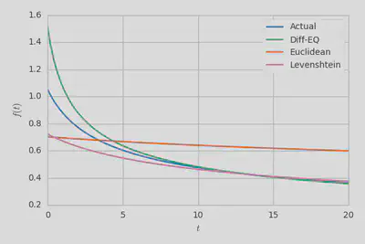
There’s clearly some significant error when $t$ is small but if you look back at the fit for this newer data then you’ll see that there was some upward curvature in $\tau(t)$ for low $t$ and that the preferred y-intercept is actually much closer to $0.888$ than $0.41$. If we had allowed for this curvature then the agreement here would be much, much better… doing so just seemed pointless given the poor quality of the $\nu(v)$ constraint. In either case, the parameterization is surprisingly accurate given that the Arc 2 code already significantly broke our assumptions and the more recent data obviously corresponds to much more extreme violations. I suspected that fuzzing-like effects would cancel to leading order when the bounds overlapped but there’s actually something more interesting going on here that explains why the agreement is so good despite the assumptions breaking down.
The value of a bound on $\tau(t_1)$ when Story 1 appears first is $v_2 \frac{t_2-t_1}{v_2-v_1}$. Adjusting the score of Story 1 upwards by some factor wouldn’t change this expression at all. Adjusting the score of Story 2 upwards such that it now appears first results in a bound on $\tau(t_2)$ that is equal to $v_1 \frac{t_2-t_1}{v_2-v_1}$. If $v_1 \approx v_2$ and $t_1 \approx t_2$ then we find that the value of the computed bound doesn’t change due to the score adjustment. Instead, only the regions over which the bound would be upper or lower change. If we’re randomly adjusting the final scores of stories by some factor then the additional contributions from upper and lower bounds exactly cancel. You don’t even need the $t_1 \approx t_2$ constraint when you consider the distribution over the whole ensemble of data.
If you look at story pairs where $v_1$ and $v_2$ are very different then this is no longer true; the value of the bound jumps discontinuously when the story order changes. This means that the density of upper and lower bounds will no longer cancel, they’ll grow with $|v_2-v_1|$, the magnitude of the adjustment factors, and how quickly the story density changes with respect to $v$ and $t$. The thing is, as $|v_2-v_1|$ grows, any measured bounds (without adjustment) get further from the real value of $\tau(t)$. The same discontinuity that causes the contributions to not cancel simultaneously reduces the overlap (or eliminates it completely depending on the size of the adjustment factor). This is a direct result of $\frac{\partial^2 \mathcal F}{\partial t^2}>0$ and our extrapolated tangent line falling under the curve. $t_1$ and $t_2$ have to have similar values to get a very tight constraint and that means $v_1$ and $v_2$ also have to have similar values.
This goes far beyond my somewhat hand-wavey original assertion that the overlap cancels to leading order.
The quality of the extracted $\tau_0$ and $\tau_1$ parameters make a lot more sense in light of this.
It also makes more sense why the $\tau(t)$ fits looked OK in the newer data but the $\nu(v)$ fits looked really bad.
The constant factors weren’t the issue, it was really the different $v$ dependence introduced by the contro-factor.
The distribution of bounds violations was sort of an admixture of one preferring a linear function and many preferring cubic functions.
Then on top of that you also have the contributions from the various adjustment factors.
In Other Words
We took a data driven approach to figuring out how the Hacker News algorithm works and were able to make some fairly accurate inferences about how the score function has depended on a story’s age and vote total at various points in the site’s history. Our methodology proved to robust against violations of our initial assumptions and generally outperformed global optimization approaches at reconstructing the parameters used in the Arc code, particularly when adjustment factors became more prevalent. It even guided us to the correct functional form for the score function while it would have been difficult to do anything beyond guess-and-check with the global optimization approach.
Overall, it was a fun problem space to explore and I hope that you enjoyed following along.
Evan Sangaline
Vice President of Artificial Intelligence
My interests include web development, machine learning, and technical writing